
SAP Analytics Cloud Compass: New Guide for Planning and Risk Analysis

Companies operate in a dynamic environment. Uncertainty is part of it. This is where the SAC Compass comes in. Users should be able to examine various future scenarios at the push of a button without statistical knowledge. But does it deliver on its promises?
Today, companies operate in a dynamic environment. Uncertainty is the order of the day. This is precisely where the SAC Compass, released in early 2025, comes in. Users are to be enabled to examine different future scenarios at the push of a button without statistical or programming knowledge. But does the Compass deliver on its promises? We took a closer look.
The SAP Analytics Cloud Compass is an integrated tool for Monte Carlo simulations. It thus extends traditional planning with a probabilistic approach. Instead of fixed planning values, users define uncertain influencing factors (e.g., sales volumes, prices, costs) as probability distributions. The system varies these parameters thousands of times, calculates the target KPI such as revenue or contribution margin, and then shows a probability distribution instead of a single value. This creates a clearer picture of how realistic individual scenarios are and what ranges to expect in planning.
It is important to know: This is not machine learning, which can make trends and predictions from historical data. The SAC Compass uses custom probability distributions based on human expert knowledge and current market assessments. The advantage: Users retain full control over assumptions. This allows for scenarios to be played out that have never occurred historically.
How does a Monte Carlo simulation work?
The underlying Monte Carlo simulation is an approach that actively incorporates uncertainty and provides a robust decision-making basis—far beyond rigid best/worst-case analyses. Generally, it proceeds in four phases:
- Define distributions:Each driver receives a statistical distribution (often normal distribution) that captures how much and to what extent values can vary around a mean.
- Draw random samples:For each simulation run, the algorithm randomly selects a value from each distribution.
- Simulate repeatedly:With several thousand runs, a distribution of the target KPI emerges, showing how the result area behaves under uncertainty.
- Analysis & thresholds:From the resulting curve, probabilities (e.g., 95% realistic range) and extreme scenarios (lower/upper 5%) as well as probabilities of achieving specific targets (e.g., 90% chance of reaching revenue X) can be read.
What the SAC Compass can really do
The SAC Compass offers the following core functionalities:
- Driver configuration:Flexibly vary influencing factors with realistic min/max values.
- Histogram & probabilities:Visualise result distributions clearly and determine probabilities of achieving defined thresholds.
- Integrated planning:Use Compass directly in SAC without additional licensing or external tools.
- Versioning & collaboration:Seamlessly save, document, and share simulation results within the team.
In practical application of the SAC Compass, there are differences to consider. Depending on the goal, a different number of simulation runs is recommended. For those seeking quick orientation for a preview, 1,000 runs should suffice. The result is expected in about 30 seconds. Standard analyses require more like 10,000 runs (with a result in about 1-2 minutes). For critical decisions, a precise risk analysis is advisable. In this case, 100,000 runs are the benchmark.
The decision regarding the selection of the underlying distribution can also make a difference in calculations. While the normal distribution is more suitable for symmetrical fluctuations (e.g., in commodity prices), the uniform distribution should only be applied when all values are indeed equally likely.
There are also pitfalls to consider in application. For example, overly narrow ranges lead to unrealistically precise results. Currently, correlations between drivers are not considered, and only absolute values are possible, but no percentage fluctuations. The latter is intended to be implemented in future expansions of the SAC Compass.
A practical example: We simulate our contribution margin
To test what the Compass can really do and simultaneously make the added value of the tool directly visible, we ran a small example and simulated our contribution margin.
Our planning model contains four accounts: Contribution Margin (CM), Fixed Costs, Variable Costs, and Quantity. The central formula is:
CM = Quantity × Price - Fixed Costs - Variable Costs
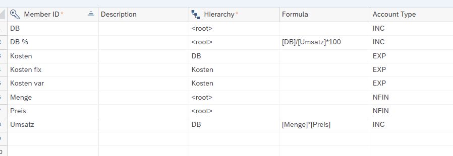
Figure 1: Extract from the model
For the SAC Compass to work correctly, certain prerequisites had to be observed in the model. Clearly defined hierarchies and formulas are essential, as otherwise the tool cannot establish logical dependencies between values. Specifically, this meant checking the account types for us, as only income (INC) and expense accounts (EXP) can be used as drivers. Additionally, an account dimension with a corresponding account hierarchy is necessary. Another technical requirement is the aggregation type 'SUM', as other types like AVG or MAX lead to runtime errors because the Compass requires additive calculations. Once the model was prepared, we defined the drivers in the next step. For this, we set a realistic range and distribution for each account in the Drivers view to practically represent typical market fluctuations and internal uncertainties.
| Treiber | Min-Wert | Max-Wert | Verteilung |
|---|---|---|---|
| Fixe Kosten | 55.000 € | 60.000 € | Normalverteilung |
| Variable Kosten | 35.000 € | 40.000 € | Normalverteilung |
| Menge | 500 Einheiten | 600 Einheiten | Normalverteilung |
| Preis | 200 € | 250 € | Normalverteilung |
In the system, it looks like this:
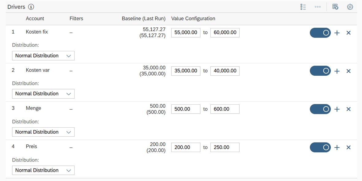
Figure 2: Driver configuration
Then simulation was conducted. Since the target KPI contribution margin represents one of our central values, we aimed for high precision, which led us to complete around 100,000 runs. The result yielded the following outcome:
- 90 % realistic range: approximately €18,900 to €38,800
- Pessimistic 5 % range: below €18,900
- Optimistic 5 % range: above €38,700
In SAC Compass, it looks like this:
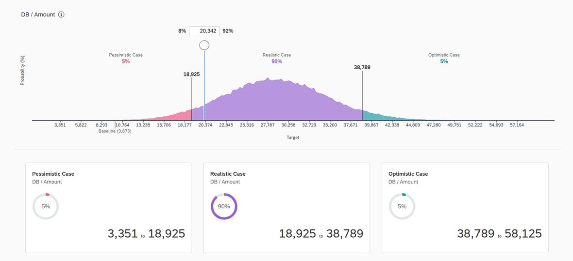
Figure 3: Results of the Monte Carlo simulation
From these results, we could derive specific recommendations for action. For risk management, this means we should prepare contingency measures in case the contribution margin falls below €18,900, which has a probability of 5%. For budget planning, the fluctuation range of ±35% in the realistic area indicates that the budget should be designed flexibly. As a decision-making aid for new projects, the 50% mark at around €28,500 provides a realistic expected value for business cases.
Bonus for us: By saving as a version in SAC, we can conveniently compare results and discuss them within the team.
Conclusion: How good is the SAC Compass
The SAC Compass makes complex simulation technology accessible to professionals and integrates it seamlessly into SAC planning. With a few adjustments in the model, scenarios can be played out and added value generated. Through the probabilistic approach, companies gain a robust decision-making basis, more transparency, and significantly higher planning certainty. Thus, the Compass—nomen est omen—serves as a reliable steering aid in a world where uncertainty has become the norm. Whether in budget planning, investment decisions, or product launches—the SAC Compass can provide crucial assistance.


